
Profit is not cash, only cash is cash as the saying goes. Cash is of course very important to any business. To be exact, cash flow is very important to a business. With credit sales and deferred payment transactions becoming dominant in business the cash balance of a business can be easily divorced from its profit. Cash management has become very important because of this. Cash management models are the brainchild of economists and accountants trying to address the problem of keeping cash balances healthy enough to meet current obligations while not keeping too much cash. There are two prominent cash management models namely Baumol’s Economic Order Quantity and the Miller-Orr cash management model.
Table Of Contents
What Is Cash Management?
Cash management refers to a system used by an organisation to steady their cash flow. As already explained payment can be deferred when goods or services are provided. On the other side suppliers and expenses will need to be met. The basic idea is to always have enough cash on hand to meet expenses. However, having too much cash on hand represents a poor cash management model. There is a cost of capital just as there is a cost of working capital. Working capital is sometimes borrowed, therefore has an outright cost of capital. Where working capital is not borrowed the cost of capital is the opportunity cost of keeping the money in a low or no interest bank account instead of putting the money in a short term investment security which pays interest. Whichever way you look at it having excess cash is also costly to an organisation.
Why Manage Cash?
For the reasons we have already outlined businesses need cash management models. The bigger the business the more it needs a cash management model. Consider a business which has an excess cash balance that averages $1 million over the year. Keeping so much cash is a sign that the business had no other places to invest the cash such as inventory. If this business used a working capital loan at 6% per annum the business pays $60000 in interest annually for cash it does not use. On the other hand, if the business financed working capital from equity so there was no interest charge for it there would still be a cost. If an instrument like a treasury bill offered 5% per annum the business loses out on $50000 it could earn from putting the excess $1 million in such an instrument. Cash management models look to address the problem raised in both scenarios. Cash management models also address the problem of not having enough cash.
Baumol’s EOQ Model Of Cash Management
In 1952 William Baumol suggested cash could be managed in the same way as inventory, through the Economic Order Quantity model. There are merits to Baumol’s ideology on cash management models. Cash can be treated as an inventory item seeing as it has a demand, a supply and a known cost. The cost is the cost (or opportunity cost) of capital. The Baumol cash management model attempts to minimise the costs associated with holding cash the same way Economic Order Quantity in inventory seeks to optimise the costs associated with holding inventory.
Assumptions
Baumol’s cash management model has four underlying assumptions;
Constant rate of cash usage
The cash management model assumes that the rate of cash usage in the business is constant. This assumption means the cash management model may not be useful in volatile times or businesses with seasonal behaviours.
The constant opportunity cost of capital
The cash management model also assumes the cost associated with purchasing and disposing of marketable securities is constant throughout the year. This is plausible but rather complex to always anticipate.
Opportunity cost
The aforementioned opportunity cost of capital is another underlying assumption of the Baumol cash management model. Therefore in the rare event that such opportunities are not available the model is not useful to businesses.
Open Market
The existence of an open market for the instrument used. Marketable securities are favoured because of their liquidity. They trade on open markets and are quickly disposable. Without the existence of such a market, the cash management model may not be applicable.
Example
According to Baumol’s cash management model, the optimum amount to be transferred each time is ascertained as follows:
C = √ (2AT/I)
Where,
C = Optimum transaction size
A = Estimate cash outgoings per annum
T = Cost per transaction
I = Interest rate on marketable securities
So if our business estimated cash outgoing per annum to be $1 million, cost per transaction to be $8000 and interest on marketable securities was 12% our Economic Order Quantity would be;
√[(2*Outgoings*Cost per transaction)/Interest Rate]
√((2*100 000*8 000)/12%)
√( 16 000 000 000/12%)
√(133 333 333 333.33)
365 148.37
Optimum transaction size is $365 000. Therefore the business would make the transaction in 3 times a year to optimise the costs associated with managing the cash balance.
The Miller-Orr Cash management Model
The other cash management model known as the Miller-Orr cash management model assumes that cash movement in a business is erratic. Payments are neither predictable in timing nor uniform in size. The same is assumed of the cash needs of the business. The cash demand is also believed to be erratic in this cash management model. This cash management model specifies three points for the cash balance of a business as follows;
The upper limit (h) is the level at which a business is holding too much cash and must reduce its cash balance by buying marketable securities or other instruments that earn interest for the cash.
The lower limit (o) is a level which the business must strive to always be above in terms of cash balances. Going below this level puts the business at risk of being insolvent.
The return point (z) is the target level of the cash balance that the business will aim for when buying instruments to reduce cash balance or selling instruments to increase cash balance.
Assumptions
The Miller-Orr cash management model has two underlying assumptions;
No underlying trend in cash
Firstly the Miller-Orr cash management model assumes there is no trend of growth or decline or cash over time. This is because the points h and z are static themselves.
Cash fluctuations
The points h and z are dependent on daily fluctuations in cash in the business. The cash management model is therefore useful in times of uncertainty and random cash flows. It also requires a fixed cost of buying and selling marketable securities to be effective.
Example
So assume our business has a lower limit of $150000, the daily interest rate is 0.033% (12%/365 days), cash flow variance $100000 and transaction cost of $100 we calculate the spread as follows
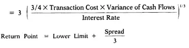
3[(3/4*Transaction Cos*Variance of Cash Flows)/Interest rate]^1/3
3((3/4*100*100 000)/0.033%)^1/3
3((3/4*10 000 000)/0.00033)^1/3
3(7 500 000/0.00033)^1/3
3( 22,727,272,727.27273)^1/3
3(2 832.58)
8 497.75
Upper limit h = spread + lower limit
H =8500+10 000
H = 18 500
Return point = lower limit + 1/3*spread
Z = 10 000+1/3*8500
Z = 10 000+2833.33
Z = 12 833.33
Baumol’s Economic Order Quantity cash management model and the Miller-Orr cash management model differ in approach but attempt to solve the same problems. The opposed problems of holding too much cash and too little cash.